Fall 2022 Alpha Competition Recap
Aditya Ranjan & Jerome Mathew
During the fall semester of the 2022-2023 school year, while many members of the group were adapting to a new organization of the verticals and working on things like design for higher frequency trading, the new members were all working toward developing their final product and presentations for the Alpha Competition. Designed by the senior members of the group, this SIF ritual prompts the junior quantitative analysts to have some tangible experience with developing alphas as well as combining various pieces of information from finance, statistics, and math that were gained over the course of several lecture series throughout the semester.
For the 2022 Alpha Competition, the analysts were allowed to use any data available from 2010-2015 to help develop their alpha. The final results would be decided based on the performance of the alpha over the in-sample time period aforementioned as well as a hidden out-of-sample period that would be hidden from the participants. The metric for performance was a combination of the overall returns, sharpe ratio, and even qualitative measures such as creativity.
As one of the new members, Jerome Mathew (another new member) and I formed one of the participating teams. With only a few days left till the competition, we were initially at a loss for ideas to develop our alpha. While I was playing around with technical indicators such as RSI and Bollinger Bands, Jerome preferred the idea of working with something more theoretical.

Low RSI values such as those below 30 can sometimes be a good indicator for local minima and are generally thought of as good buying indicators since the price is undervalued. For example, in the image below, the price of a certain stock is depicted where RSI values under 30 are highlighted in red. These all seem to be decently good buying points for an algorithm.
Allocating all funds to one stock with the lowest RSI is risky and doesn’t often perform as expected. Dividing the funds among some N number of stocks with the N lowest RSIs in a selected universe is a better strategy to help diversify against risk. However, the question then becomes what weights should be set for each ticker so that it performs optimally?
This is where we incorporated the Markowitz Efficient Frontier. In one of the lectures on financial models, we learned about the efficient frontier portfolio that is used to maximize returns for the amount of risk or standard deviation in returns. More specifically, there was a code example (credit to Steven Struglia) that implemented this to show how it can be used practically as well. This involved generating a lot of random weights in a portfolio and then using past daily returns as well as the covariance of returns to calculate the sharpe ratio for each of these weights. For example, below is an image showing the results of 80,000 randomly generated weights for a portfolio of the 7 stocks with lowest RSI values on a given day.
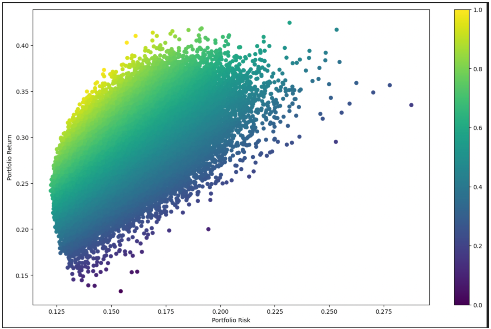
We decided to go with a portfolio of 7 stocks as the frontier seemed to be a smooth curve as we expected. After increasing the portfolio size beyond that, the graph shape was very irregular and not similar to what it should look like theoretically. This could be because the weights search space was not being scanned enough for such a large portfolio, but we also didn’t have time to implement other techniques such as convex optimization to solve the problem. However, this is something we would like to take a look at later.
After backtesting the alpha, we were pleasantly surprised to see that the alpha performed very well on both the in-sample and out-of-sample time periods of 2010-2015 and 2000-2005 respectively, winning the competition! Below are the results, highlighted in blue and labeled rsi_mark.


